Date: December 31st, 2020
Class: DS 320
Instructor: Marc Rigas (Penn State University, College of Information Sciences and Technology)
Introduction
In this phase of the semester project our objective was to practice using data science techniques to extract and clean data, and then to integrate data using implementations of some of the techniques we learned in class.
In part A of phase 2 we cleaned the data, identified missing values, and formally assessed the similarity of the data using instance-based matching.
In part B we used FlexMatcher to match columns of different coronavirus datasets together.
Link to code here.
Data Description
Our group used a multitude of datasets. We did not use the same data that we used for part 1. For part A we used fast food location datasets, one from data.world which focused on subway restaurant locations, and another from Kaggle which used a variety of fast food restaurant’s locations such as McDonalds, Wendy’s, etc.
We used the drop_duplicates() function on both datasets once they were converted into dataframes, and after comparing the shape of both the original and the dropped duplicate dataframes, the number of records was the same, so we concluded that there were no duplicates.
To determine where the missing values were we used the count function to count the cells in each column that had non-missing values and compared that to the total number of records.
As you can see from the number of records compared to the count of non-missing values, the dataworld dataframe, the url, phone_number, fax, email, website, facebook, twitter, instagram, pinterest, and youtube values all have missing values. Some of these attributes had all missing values, so we decided to remove them. We did not remove the column website because we thought it would be interesting to have later on for the jaccard similarity matching. We removed 12 attributes in total.
In the kaggle dataframe on the other hand the only attribute that had missing values was websites.
We replaced the missing values with an arbitrary value ‘X’, as we thought a random variable would be appropriate as a replacement for missing values.
The attributes for the datasets are as follows.
Data.world Restaurant Locations - 11 attributes, 25,533 records
address - the address of the restaurant
city - the city the restaurant is located in
country - the country the restaurant is located in
keys - the API key used to access the information in the entity
latitude - the latitude location of the restaurant
longitude - the longitude location of the restaurant
name - the name of the restaurant
postalCode - the zipcode of the restaurant
province - the state the restaurant is located in
websites - the website url of the website related to the restaurant
Kaggle Fast Food - 10 attributes, 10,000 records
name: represent name of the restaurant,
url - used to find the information for the other attributes such as city, state, etc.
street_address - is the street address of the restaurant,
city - is the city the restaurant is located,
state - the state the restaurant is located in,
zip_code - the zip code of the restaurant,
country - the country in which the restaurant is located in,
phone_number* - is the phone number of the restaurant,
fax* - is the fax of the restaurant, email is the email of the restaurant,
website - is the website of the restaurant,
open_hours - is the hours the restaurant is open,
latitude: is the latitude number the restaurant is located at,
longitude - is the longitude number the restaurant is located at,
facebook* - is the link for the facebook page of the restaurant,
twitter* - is the link for the twitter page of the restaurant,
instagram* - is the link for the instagram page of the restaurant,
pinterest* - is the link for the pinterest page of the restaurant,
youtube* - is the link for the youtube page of the restaurant.
Asterisk = Dropped Attributes
For part B we used the John Hopkins repository discussed in the assignment prompt. From the US daily covid cases reports datasets we chose the July 11th and December 2nd cases. We chose days that would have had spikes from major holidays for fun. We then used the time series data from the same prompt and ran flexmatcher on the daily covid cases datasets to train the schema matcher and then did a prediction for the times series data. Since this an instanced based match we do not need the attributes from the time series data for testing, so we dropped them.
The time series data had 3339 records, and 330 attributes. The July 11th data had 58 records and 18 attributes. The Dec 2nd data had the same number of records and attributes compared to the July 11th dataset. There were also no duplicates after dropping the duplicates using the drop_duplicates function. We show this using the number of records before the drop and after the drop. Looking below you can see that they are the same.
Links for the different data are below.
US Daily Covid Cases July 11th
Part A: Jaccard Similarity Measure
Methods A
Comparing the column names some are the same such as name, city, latitude, and longitude, totaling to 4. That leaves 7 attributes that are different for dataworld and 6 for kaggle. Some of the names are completely different from their counterparts such as state in the kaggle dataframe compared to province from the kaggle dataframe. Therefore we decided to use instance-based matching for the jaccard.
Moving along we compared the performance between using the total word, 2-grams, and 3-grams. In order to get grams we had to create a function that could make the tokens which is shown below. The function is changed depending on whether we wish to create 2-gram or 3-gram tokens. The 3-token code is commented out.
# 2-gram
def getGrams(array):
  grams = []
  for text in array:
      # pads the text to show beginning and end of string
      text_padded = "$" + str(text) + "$"
      #text_padded = "$$" + str(text) + "$$"
      # traverses through the string and takes n-grams
      length = len(text_padded) - 1
      #length = len(text_padded) - 2
      for i in range(length):
          first = text_padded[i]
          second = text_padded[i+1]
          #third = text_padded[i+2]
          gram = first + second #+ third
          grams.append(gram)
      # appends gram to list of grams
  return grams
An example of the jaccard script for 2-gram tokens with comments explaining the steps are below. The script is the same for 3-gram besides the commented lines being changed with its associated counterpart for the 2-gram. For word tokens the lines with the gram token function are removed.
# Jaccard Similarity Measure - 2gram
# Take the set of all the tokens
col_vals = set(getGrams(kaggle_clean['address'].unique()))
jaccard_list = []
names = {}
# Get the jaccard similarity score for each attribute of dataworld compared to address from kaggle and save it
for col in dataworld_clean.columns:
    ext_col_vals = set(getGrams(dataworld_clean[col].unique()))
    intersection_size = len(col_vals.intersection(ext_col_vals))
    union_size = len(col_vals.union(ext_col_vals))
    jaccard = intersection_size / union_size
    jaccard_list.append(jaccard)
    names[jaccard] = col
# Take the maximum similarity score from the jaccard similarity score list
maxed = max(jaccard_list)
# if the maxed is not zero print the similarity score, otherwise all of the similarity scores are 0
if maxed != 0:
    print(names[maxed] + ' has similarity score ' + str(maxed))
else:
    print("All similarity scores are 0")
Results A
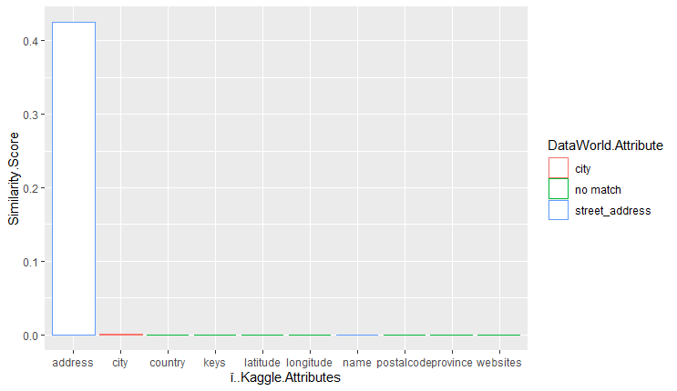
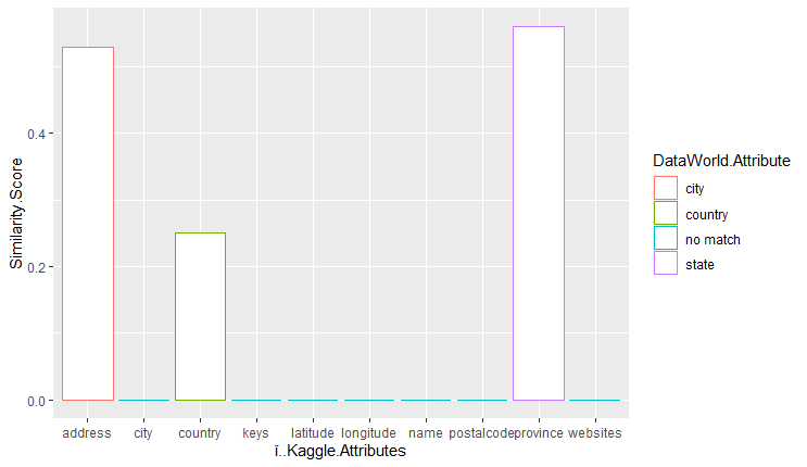
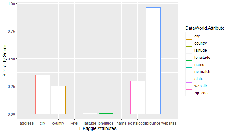
The results of the attributes of the kaggle dataframe vs the similarity score are shown below. These charts were generated by ggplot in R. The highest similarity score result with the attribute from the dataworld dataset is encoded using color. Note that even if the bar is almost negligible it is not 0 if the color is not encoded to ‘no match’ in the color legend.
3-token similarity measure:

2-token similarity measure:

Word token similarity measure:

Conclusion A
From the results we conclude that the word token jaccard performed the best, with eight out of ten attributes in the kaggle dataframe having the highest similarity scores with the most similar attribute in the dataworld dataframe. Out of those eight, four of them had significant similarity scores. I consider a similarity score to be significant if it is greater than 0.125.
The 2 token jaccard performed second best, with three out of ten attributes in the kaggle dataframe having the highest similarity scores with the most similar attribute in the dataworld dataframe. All of them had significant similarity scores. Interesting to note is that address from the kaggle dataframe matched with city instead of street_address. We attribute this to address being mostly made up of letters, and city is an attribute that is mostly letters, so perhaps values for street_address from the dataworld dataframe had more numbers in the address compared to the address from the kaggle dataframe.
The 3 token jaccard performed the worst, with only two out of ten attributes in the kaggle dataframe having the highest similarity scores with the most similar attribute in the dataworld dataframe. The only significant attribute was address, being related to street_address from dataworld.
From our initial thoughts it was surprising that the 2 token and 3 token jaccards performed so poorly in comparison to the word token jaccard similarity measure. We also found it hard to believe that the similarity score for some of the attributes in the 2 and 3 tokens could be 0. One explanation could be that for all of the values of one attribute in kaggle they are all different enough in the corresponding attribute in dataworld so that the similarity score would be 0.
Part B: Schema Matcher using FlexMatcher
Methods B
When we trained the schema matcher we ran into a problem where flexmatcher doesn’t like dealing with numbers as it applies the .lower() function at some point in the method. As such we had to turn the attributes into strings using the .astype(str) function. After this it ran with lots of warnings but still returned some results. We also had to change the version of pandas to 0.25.1 because FlexMatcher uses the ix method from a previous version of pandas. The schema list had the dataframes for daily covid cases from July 11th and December 2nd. We then got the dictionary of those dataframes to put in the mapping list, and then we put them into the FlexMatcher method with parameter sample size set to 500 to train our schema matcher. The code and the results are shown below.

Results B
After this we ran the schema matcher model on the time series dataset and returned these results.
predicted_mapping = fm.make_prediction(covid_cases.astype(str))
predicted_mapping
From looking at FIPS in the covid daily cases schema, it appears to be an incorrect match as the 0’s in the time series schema are from deaths, and FIPS does not refer to the death count per day.
Comparing the values when looking at the time series csvs and the daily cases csvs Active is not a great match, with most values being integers in the tens of thousands range, while the values in time series corresponding to 1001 are all 4 digit integers.
Deaths are correctly matched to the death number columns in time series.
Last_Update is completely incorrect as it is a date and time measurement, while it is matched to a death column in the time series schema.
The same can be said for Case_Fatility Ratio is also incorrectly matched as it is a number close to 1 in the covid daily cases schema while it is matched to a death column.
People_hospitalized has missing values while it is matched to the deaths column so that is also not accurate.
Recovered, Testing_Rate, Total_Test_Results, Incident_Rate, and Confirmed are also matched to a deaths column when it is in the hundreds of thousands range.
Latitude, Long_, Province_State, Country_Region, ISO3, and UID are correctly matched with their counterparts in the time series schema.
Interestingly Hospitilization_Rate from the daily covid cases schema was matched with what appears to be cities from the time series schema.
Conclusion B
From this particular schema match we learned that sometimes the matcher randomly picks things to match, such as the Hospitilization_Rate from the daily covid cases schema matching with the cities. With regards to schema matching in general it is very good at distinguishing unique values in columns from the testing data and correctly matching them to the correct attribute from the training data. The magnitude of a number also does not matter much when matching, as that is not taken into much consideration as they are considered as strings instead of numbers by the schema matcher.
The results were not what we expected, mostly because we were unsure about how some of the attributes from the time series schema would be matched with the daily covid cases schema. Afterwards we observed that while the schema matcher is good at identifying an attribute correctly when it is unique, it struggles when there are multiple columns in the testing data that are similar to one attribute in the training data. In conclusion, we speculate that this is because of the lack of uniquely similar values present in the training schema in comparison to the testing schema.